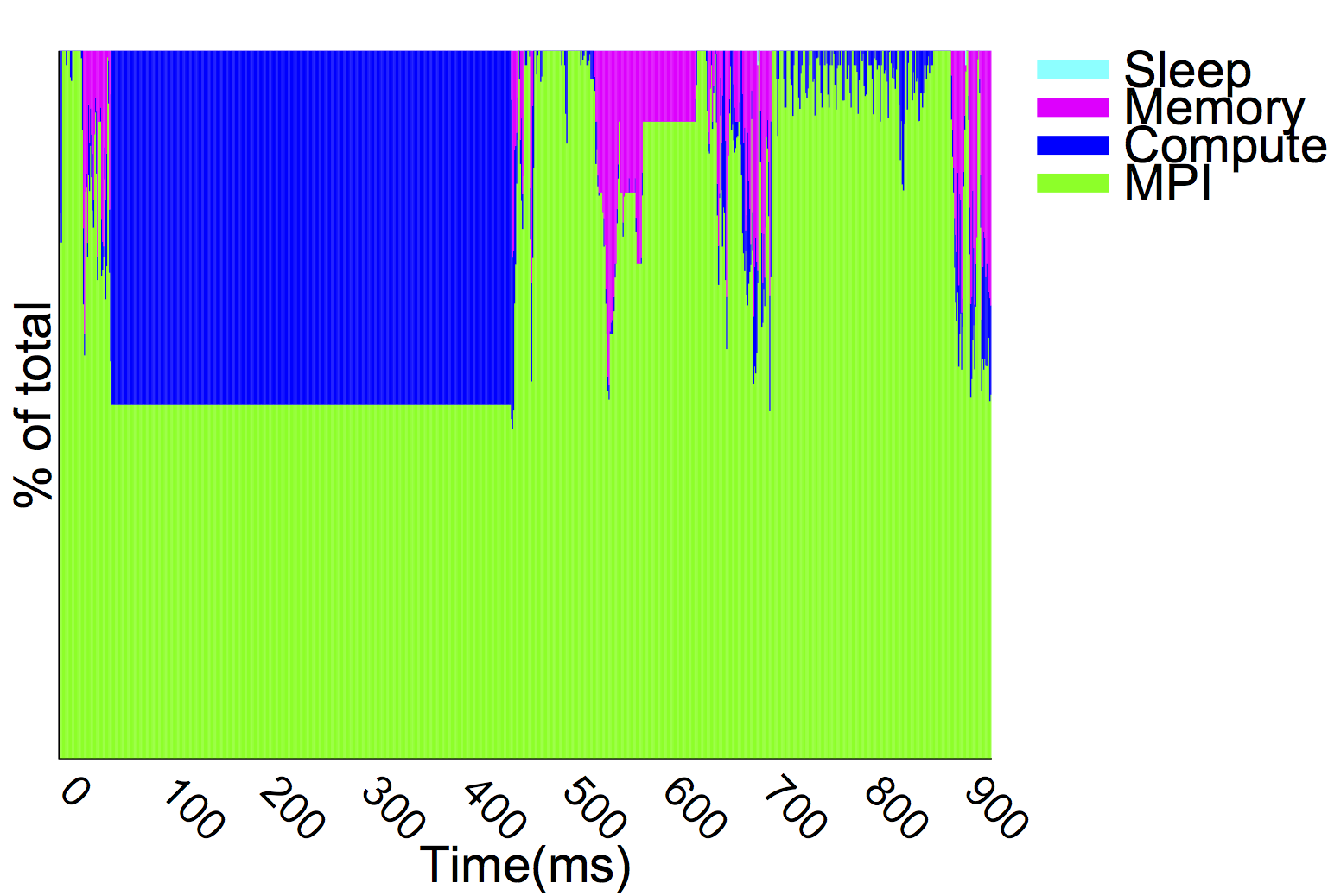
Figure 17: Application Activity (Fixed-Time Quanta; FTQ) for Simple MPI Test Suite

Fixed-Time Quanta Charts

Another way of visualizing application activity is a fixed-time quanta (FTQ) chart. While the call graph gives a very detailed profile of what code regions are most important for the application, they lack temporal information. The FTQ histogram gives a time-dependent profile of what the application is doing (Figure 17). This can be useful for observing the ratio of communication to computation. It can also give a sense of how "steady'' the application is, i.e. if the application oscillates between heavy computation and heavy communication or if it keeps a constant ratio. In the simple example, Figure 17, we show the FTQ profile of a simple MPI test suite with random computation mixed in. In general, communication (MPI) dominates. However, there are a few compute-intensive and memory-intensive regions.

The FTQ visualization is activated by another input parameter

1 ftq_trace = true

After running, two new files appear in the folder: plot_app1.p and ftq_app1.dat. plot_app1.p is a Gnuplot script that generates the histogram as a postscript file.

1 gnuplot plot_app1.p > output.ps

Gnuplot can be downloaded from http://www.gnuplot.info or installed via MacPorts. We recommend version 4.4, but at least 4.2 should be compatible.

The granularity of the chart is controlled by the ftq_epoch parameter in the input file. The above figure was collected with

1 ftq_epoch=5us

Events are accumulated into a single data point per "epoch.'' If the timestamp is too small, too little data will be collected and the time interval won't be large enough to give a meaningful picture. If the timestamp is too large, too many events will be grouped togther into a single data point, losing temporal structure.